Covid 19 epidemics in Chile: how much excess and competitive mortality?
Aims
To describe the excess mortality 2020 compared to the 15-19 period according to the month of occurrence.
To compare the differences in excess mortality according to sex, age, region, county
To compare the distribution of deaths by causes between 2020 and the previous five-year period
To study the magnitude of the effect of competitive mortality due to COVID with respect to other causes of death.
Methods
Data was obtained from the Ministry of Health Department of statistics (http://deis.minsal.cl) with the cummulative mortality registries from 1 Jan 2016 till 31 Dec 2020. We combined historical counts of mortality data from the Chilean Vital Statistics Death Database 1990-2015 and 2016-2020. From this dataset, we selected the years 2015-2019 to estimate the expected death weekly counts. Data 2020 was used to compare with the expected values. Expected deaths are estimated for all weeks of 2020 up until the week ending Dec 31, 2020.
Excess deaths are typically defined as the number of persons who have died from all causes, in excess of the expected number of deaths for a given place and time. Data from Jan 2016 till Dec 2019 was used to estimate the Weekly expected value and its upper and lower range, using three different methods :
Method 1: average with 95% confidence interval.
Method 2: median with min and max.
Method 3: overdispersed Poisson regression models with spline terms to account for seasonal patterns and its upper bound of the 95% prediction interval. The model fitted weekly death count data spanning a reference time of four years (2016-2019). The overdispersed Poisson regression models were adjusted using the farrington Flexible function from the Surveillance package. This model is based in an infectious disease detection algorithm developed by Farrington et al. The overdispersed Poisson generalized linear model includes a linear time trend and a seasonal factor to fit the data. The seasonal pattern across weeks repeated each year is included in the model, including a zero-order spline term with 11 knots, which describe 10 periods within each year. The 10 periods are split between a single 7-week period corresponding to the current week being estimated and the 3 preceding and subsequent weeks, and 9 other 5-week periods corresponding to the rest of the year. The bootstrapping method was used to estimate the 95% CI of the expected values (10,000 samples were modeled).
For each method, we estimated the number of excess deaths (i.e., observed numbers above each threshold) and percentage excess (also known as p-score, calculated as excess deaths divided by average expected number of deaths).
Using the mortality codes (XXXX) we estimate excess with and without confirmed and suspected COVID-19.
We stratified the p-score analyses by administrative regions, age and sex. In order to identify which of the causes of death increased or decreased in 2020 we stratified the analyses by causes of death.
All analyses were conducted in R.
2015-2019 fitted vs observed
plot(df0_2015_2019_w$fit, type="l")
lines(df0_2015_2019_w$value, col=2)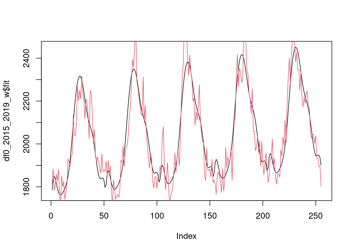
2020 expected vs observed
plot(farr_df$observed, type="l", lwd=2)
lines(farr_df$expected, col=2)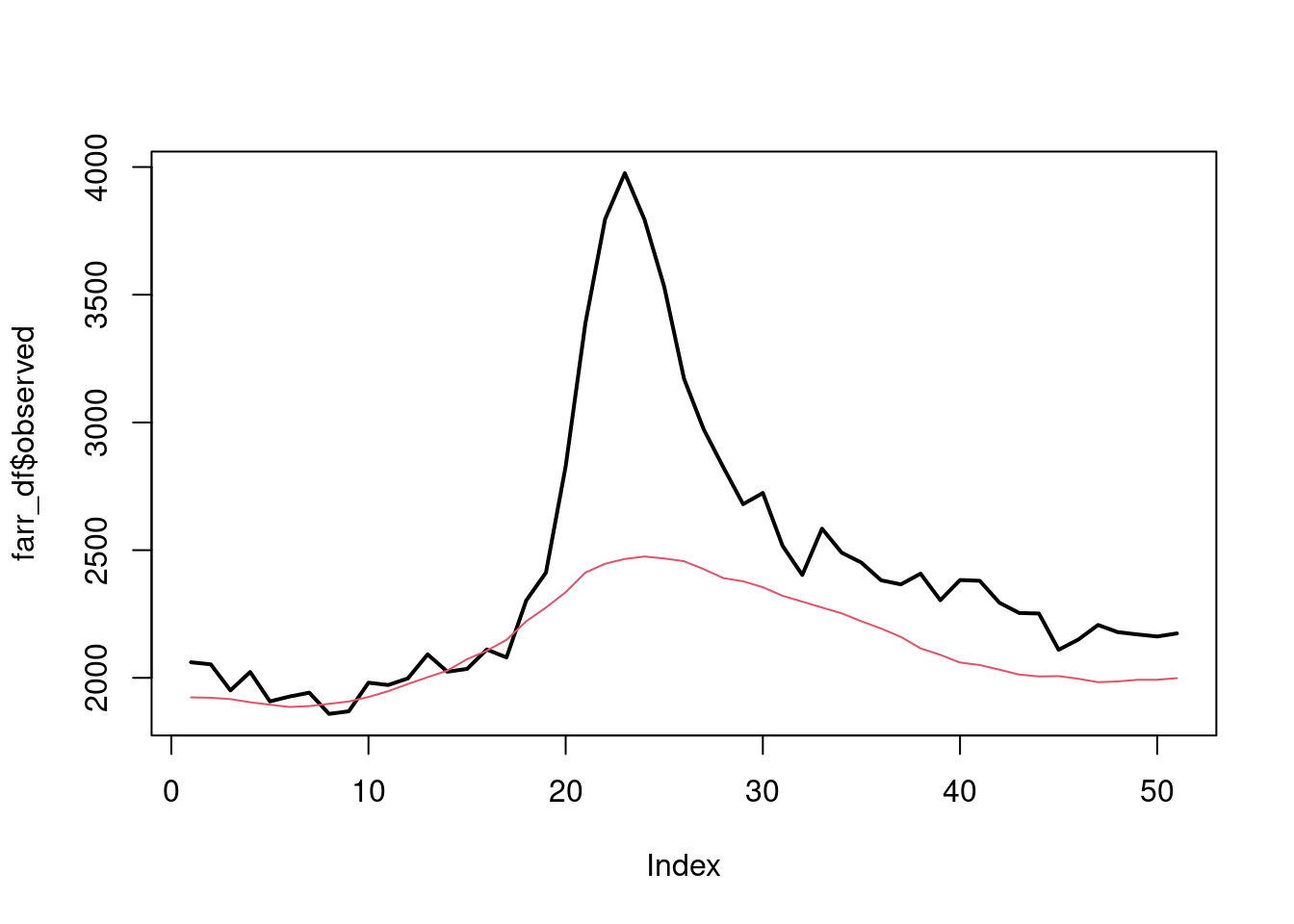
# ANOVA entre los modelos
# step(model2_ns2)
# model2_ns4 <- with(df0_2015_2019_w,
#                    glm(value ~ Date_w_coor + bs(Date_w,20),
#                                         quasipoisson(link="log")))
# summary(model2_ns4)

Predict_data<- data.frame("Date_w_coor" = 265:(265+50), "Date_w" = 1:51)

predicted_table <- predict(m2,
                           newdata = list(
                             Date_w_coor = Predict_data$Date_w_coor,
                             Date_w= Predict_data$Date_w),
                           se=TRUE)


plot(farr_df$observed, type="l", lwd=2)
lines(farr_df$expected, col=2)
lines(exp(predicted_table$fit), col=4)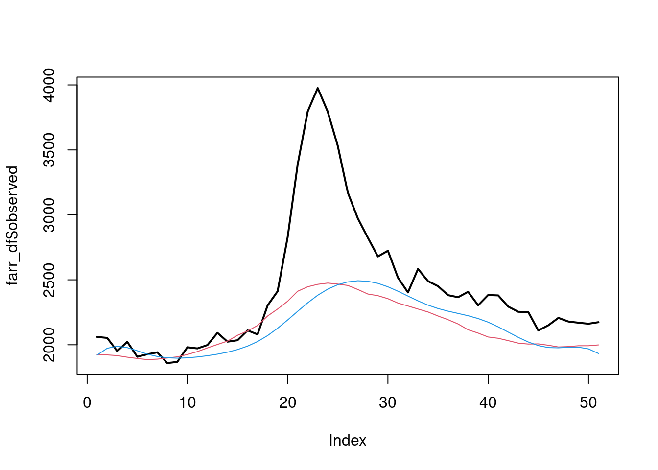
# plot(exp(df0_2015_2019_w$value))AUTO ARIMA
## Registered S3 method overwritten by 'quantmod':
##   method            from
##   as.zoo.data.frame zoo
##
## Attaching package: 'forecast'## The following object is masked from 'package:surveillance':
##
## ses## Don't know how to automatically pick scale for object of type ts. Defaulting to continuous.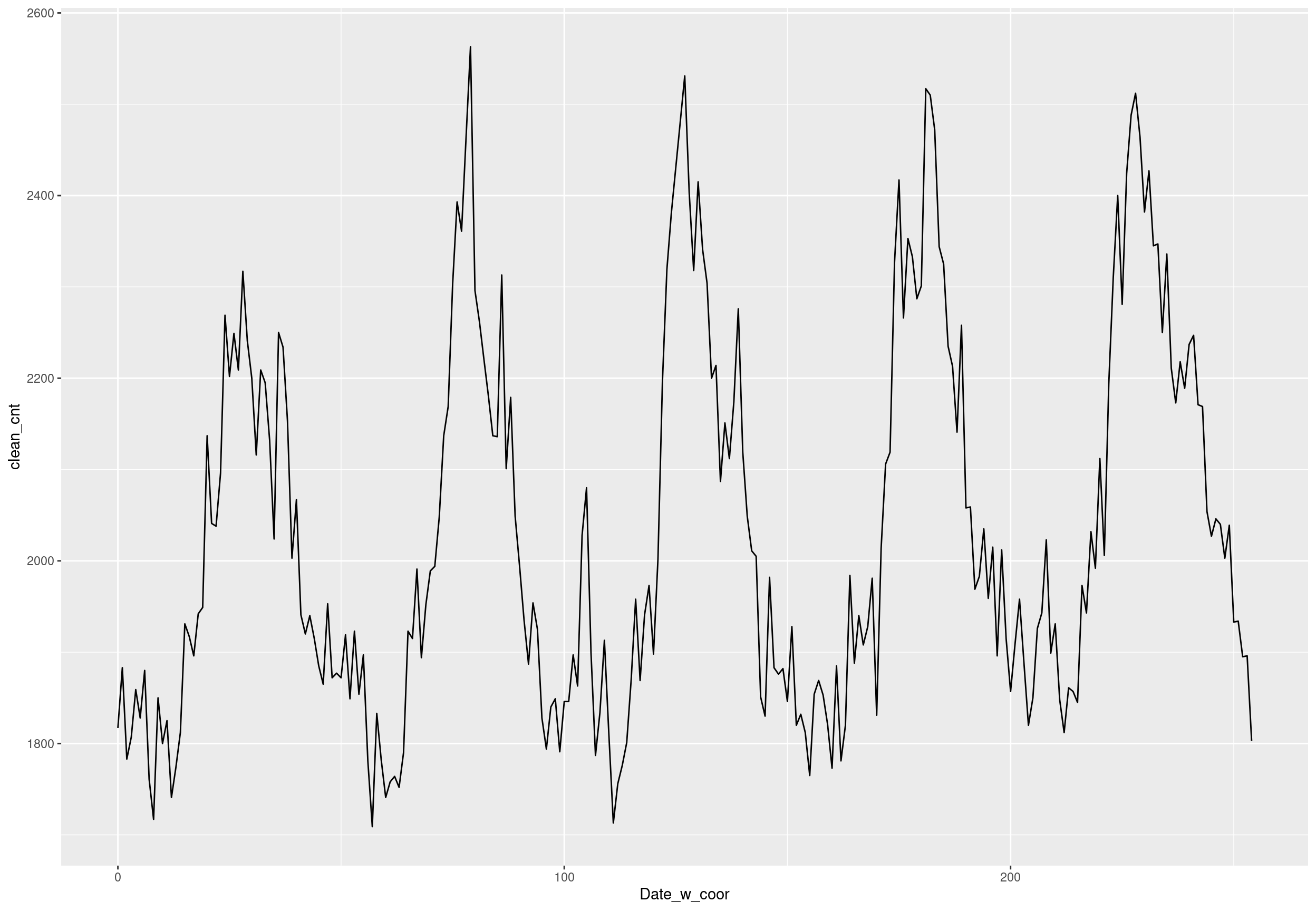
## Don't know how to automatically pick scale for object of type ts. Defaulting to continuous.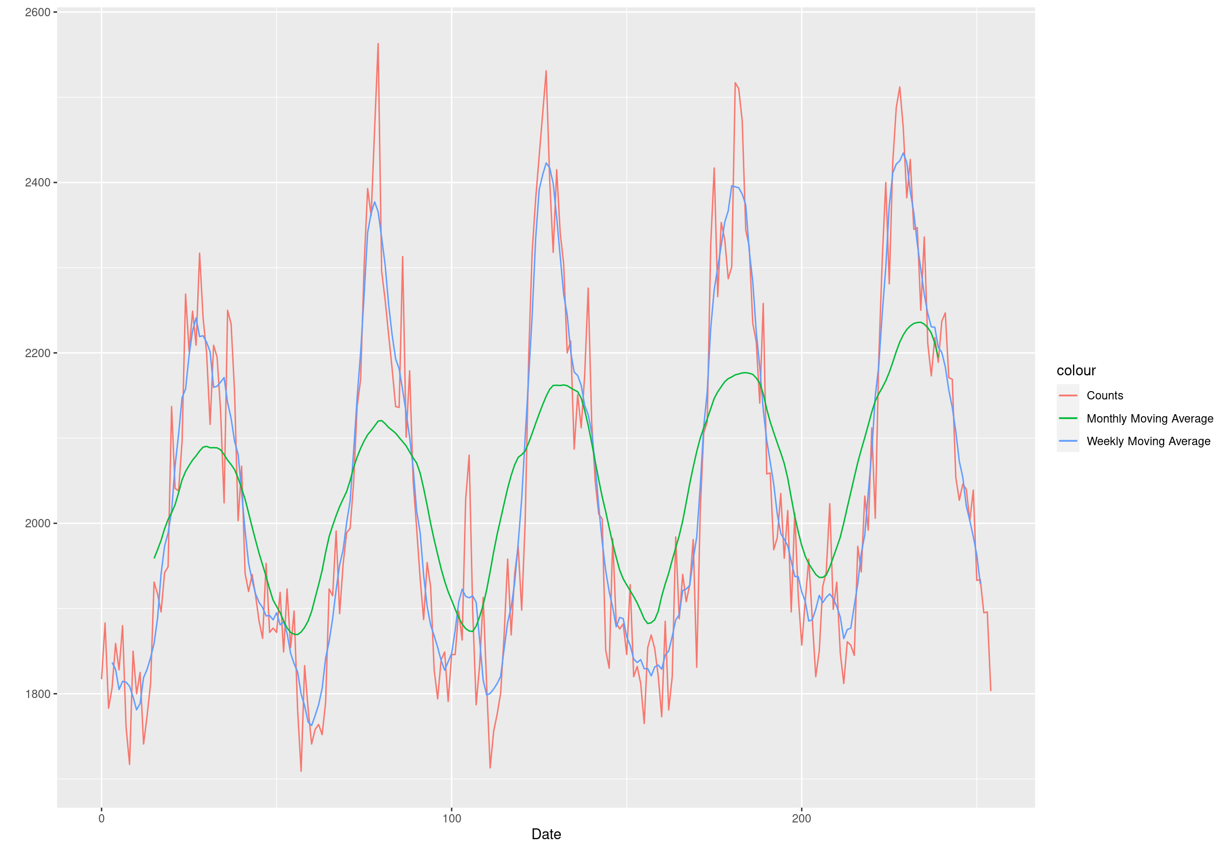
##
##  Augmented Dickey-Fuller Test
##
## data:  count_ma
## Dickey-Fuller = -4.4026, Lag order = 6, p-value = 0.01
## alternative hypothesis: stationary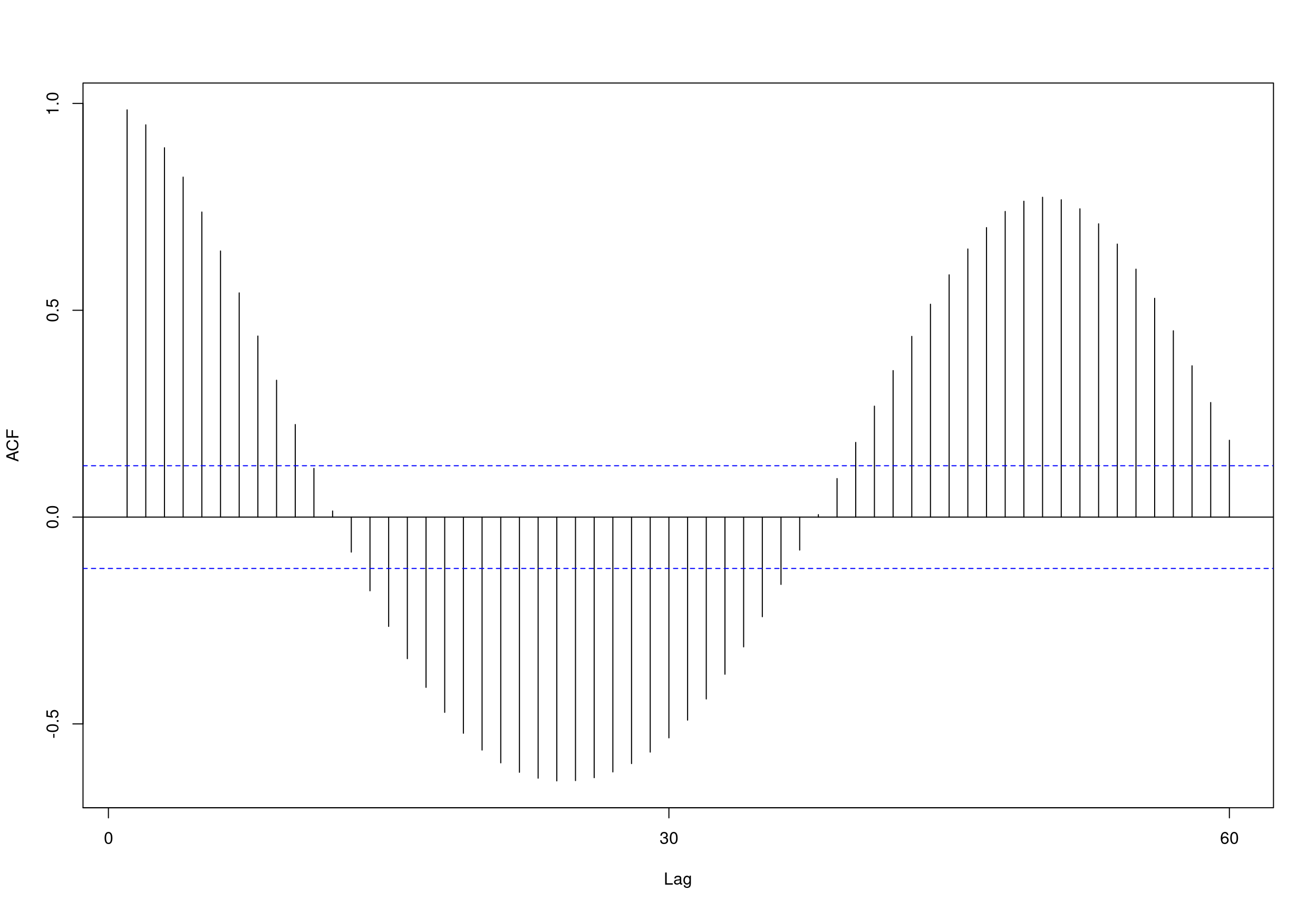
##
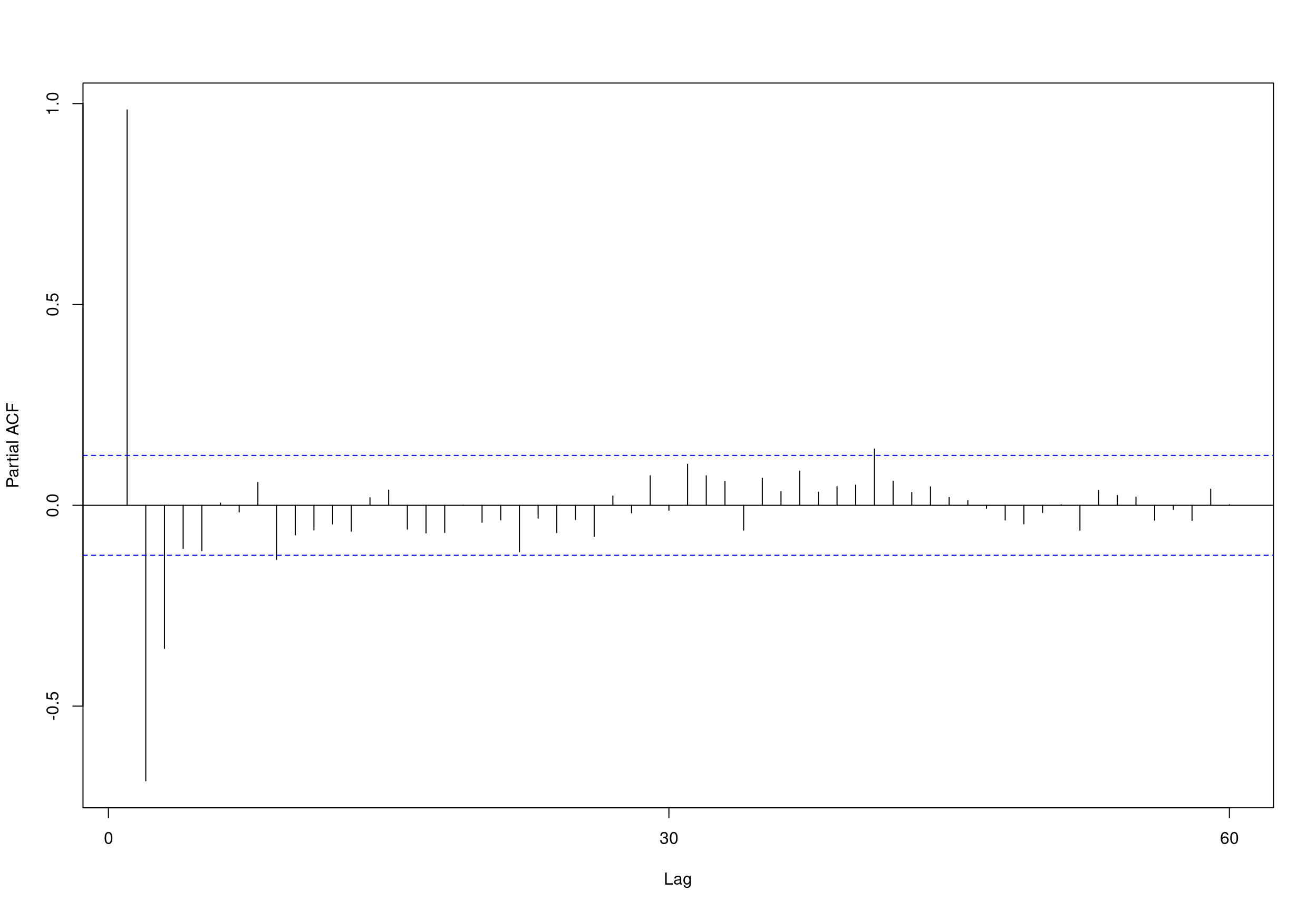
## Augmented Dickey-Fuller Test
##
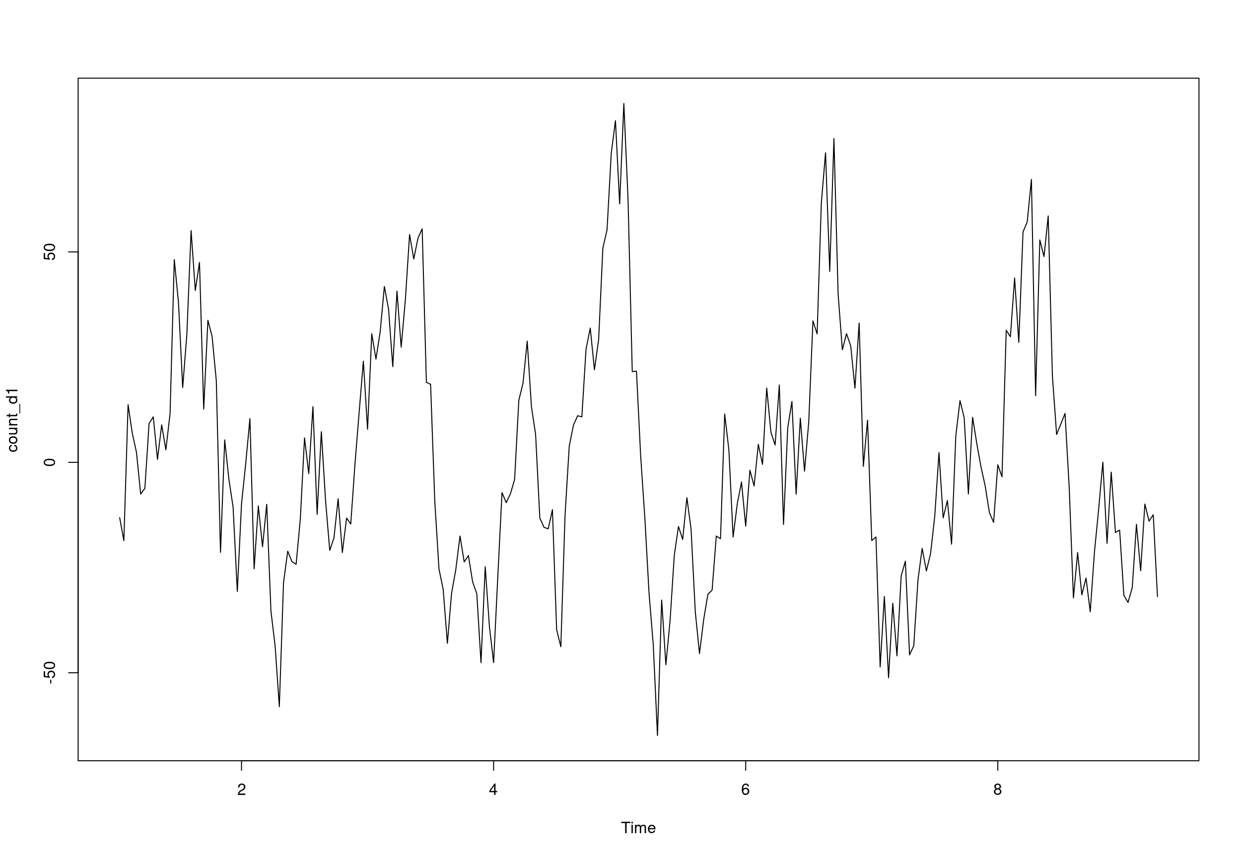
## data: count_d1
## Dickey-Fuller = -5.6459, Lag order = 6, p-value = 0.01
## alternative hypothesis: stationary
## Series: deseasonal_cnt
## ARIMA(5,1,3)
##
## Coefficients:
##          ar1     ar2      ar3     ar4      ar5      ma1     ma2     ma3
##       1.0596  0.0256  -0.7563  0.6121  -0.1383  -0.4409  0.0342  0.7465
## s.e.  0.1007  0.1447   0.1248  0.0853   0.0778   0.0857  0.0923  0.0838
##
## sigma^2 estimated as 194.6:  log likelihood=-1003.81
## AIC=2025.62   AICc=2026.38   BIC=2057.24
##
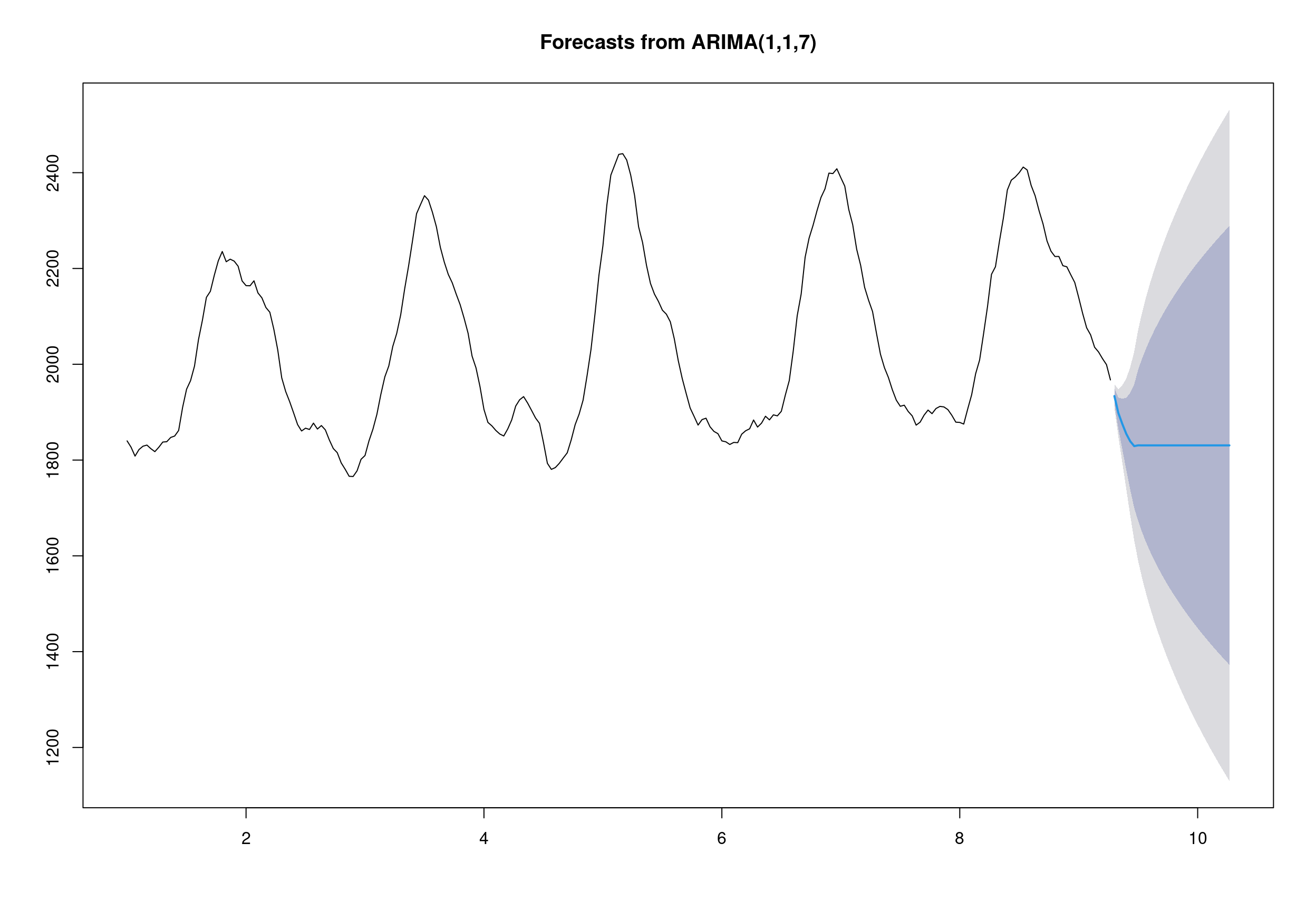
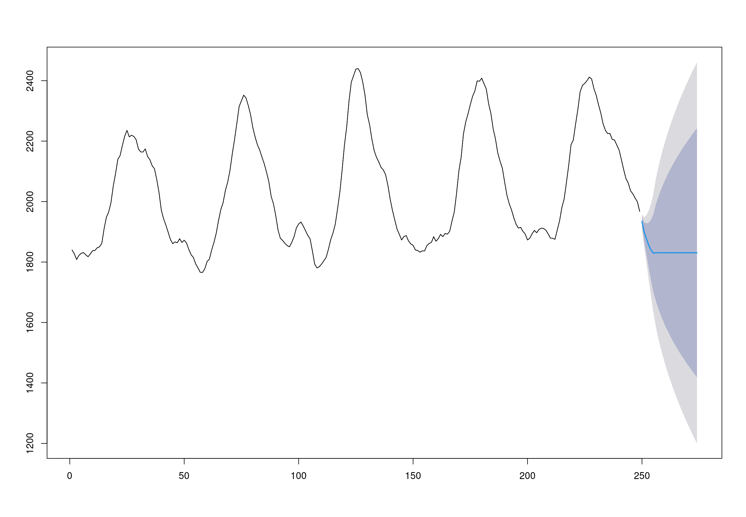
## Call:
## arima(x = deseasonal_cnt, order = c(1, 1, 7))
##
## Coefficients:
## ar1 ma1 ma2 ma3 ma4 ma5 ma6 ma7
## -0.0703 0.7773 0.9084 0.8052 0.8759 0.8173 0.7582 -0.0624
## s.e. 0.3217 0.3178 0.2544 0.3008 0.2765 0.2930 0.2845 0.2514
##
## sigma^2 estimated as 162.1: log likelihood = -987.59, aic = 1993.18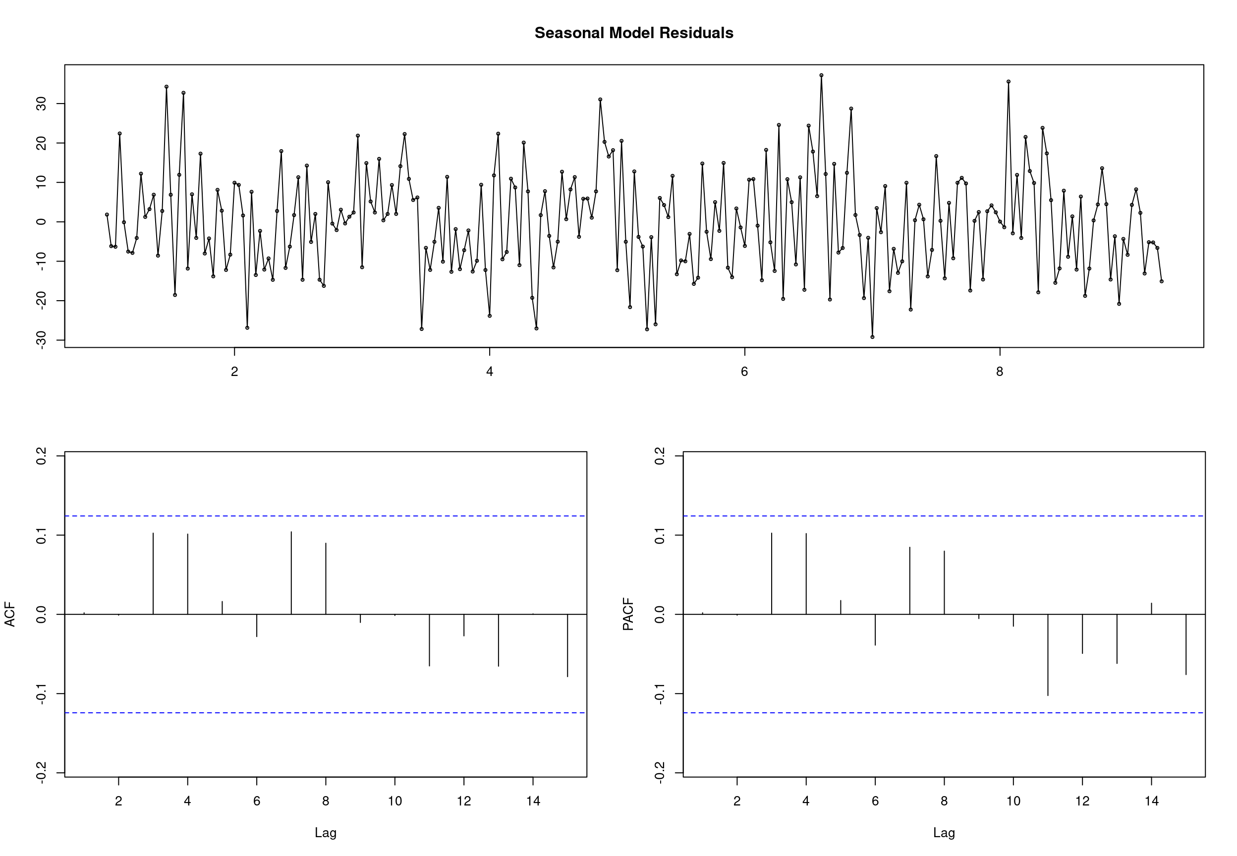
## Series: deseasonal_cnt
## ARIMA(2,1,2)(1,0,0)[30] with drift
##
## Coefficients:
##          ar1      ar2      ma1     ma2     sar1    drift
##       1.6320  -0.7123  -1.0598  0.4560  -0.1565  -0.0440
## s.e.  0.1152   0.0982   0.0945  0.1063   0.0735   4.0444
##
## sigma^2 estimated as 224.6:  log likelihood=-1021.37
## AIC=2056.75   AICc=2057.21   BIC=2081.34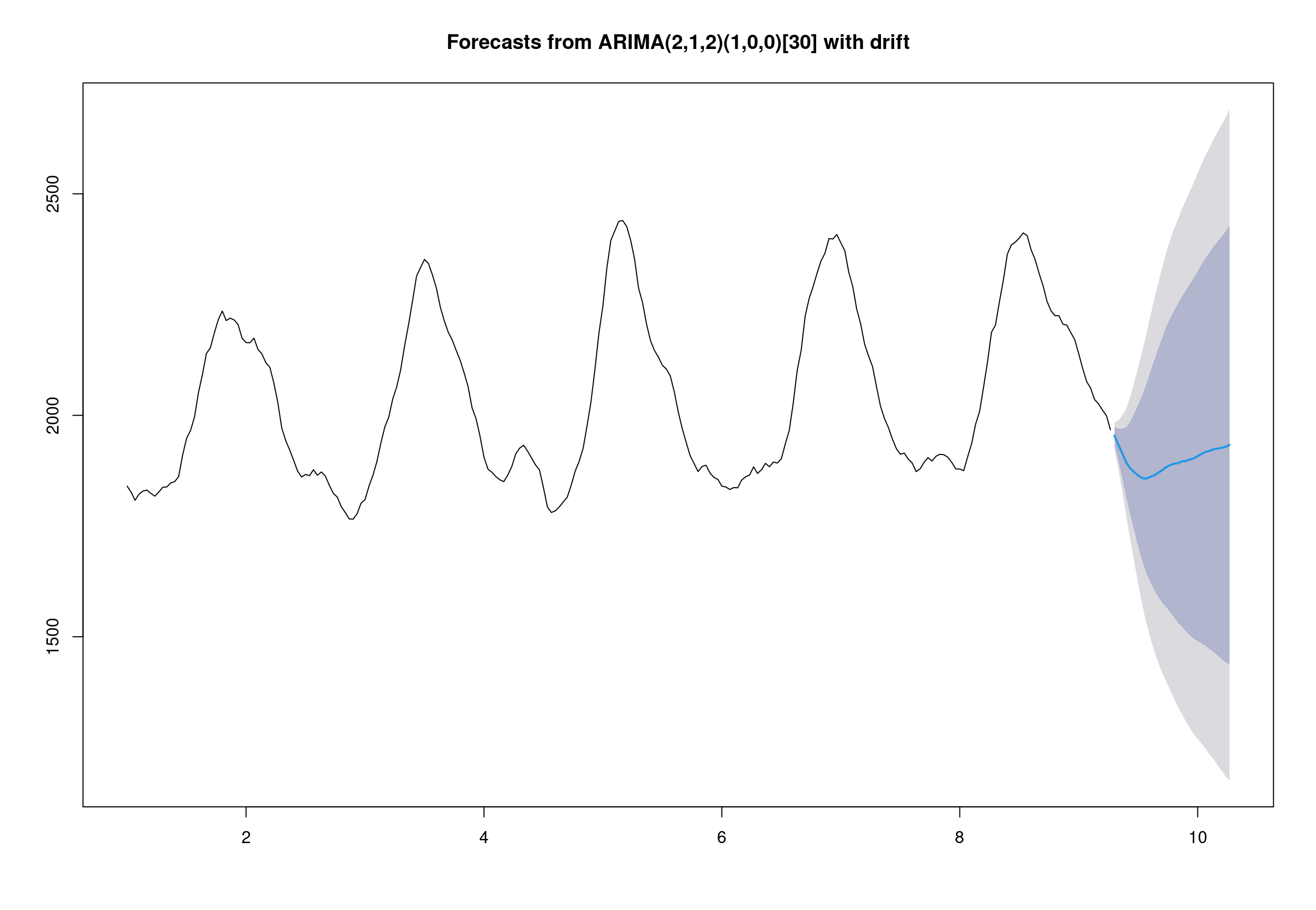
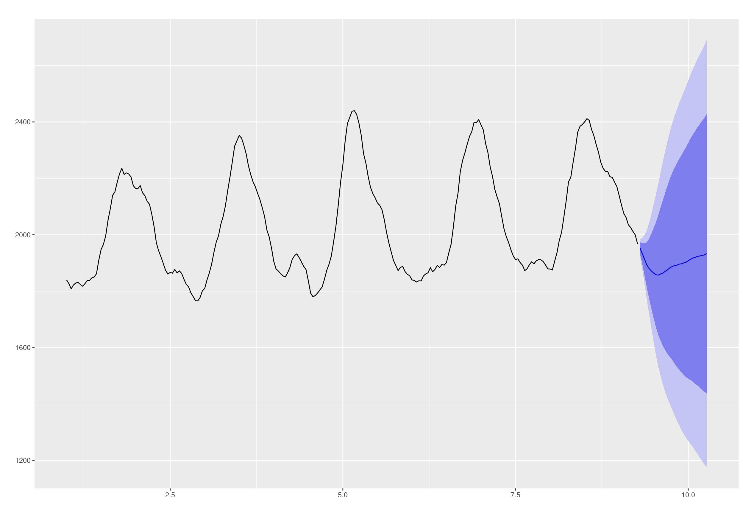
Figure 1: Weekly numbers of deaths from all causes and from all causes excluding COVID-19 relative to the average expected number and the upper bound of the 95% prediction interval. Chile, 1 Jan -26 Dec of every year 2015 - 2020
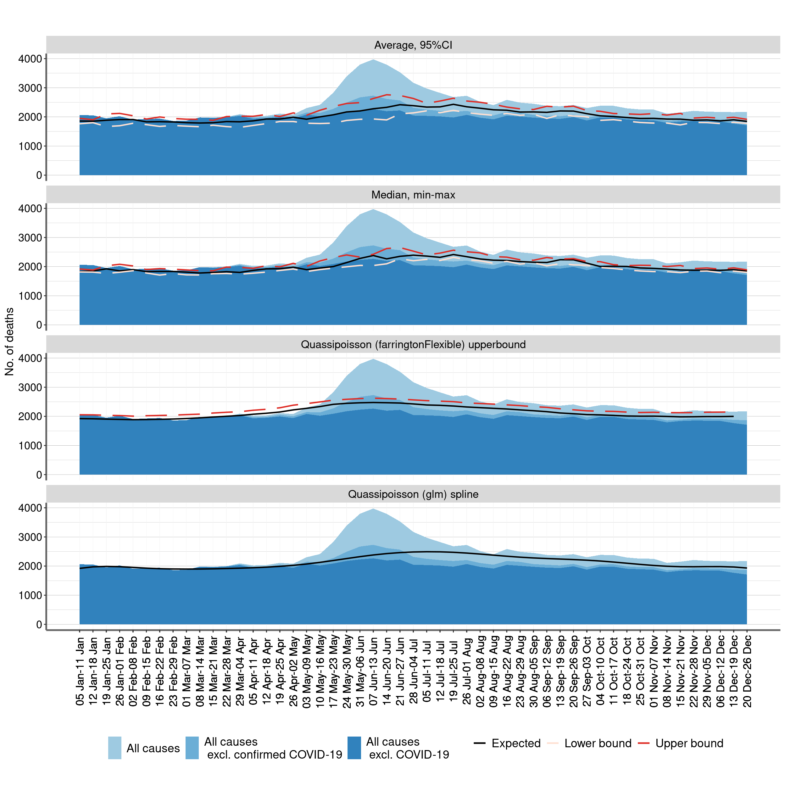
Figure 2: Weekly numbers of deaths from all causes and from all causes excluding COVID-19 above the average expected number and the upper bound of the 95% prediction interval . Chile, 1 Jan -26 Dec of every year 2015 - 2020
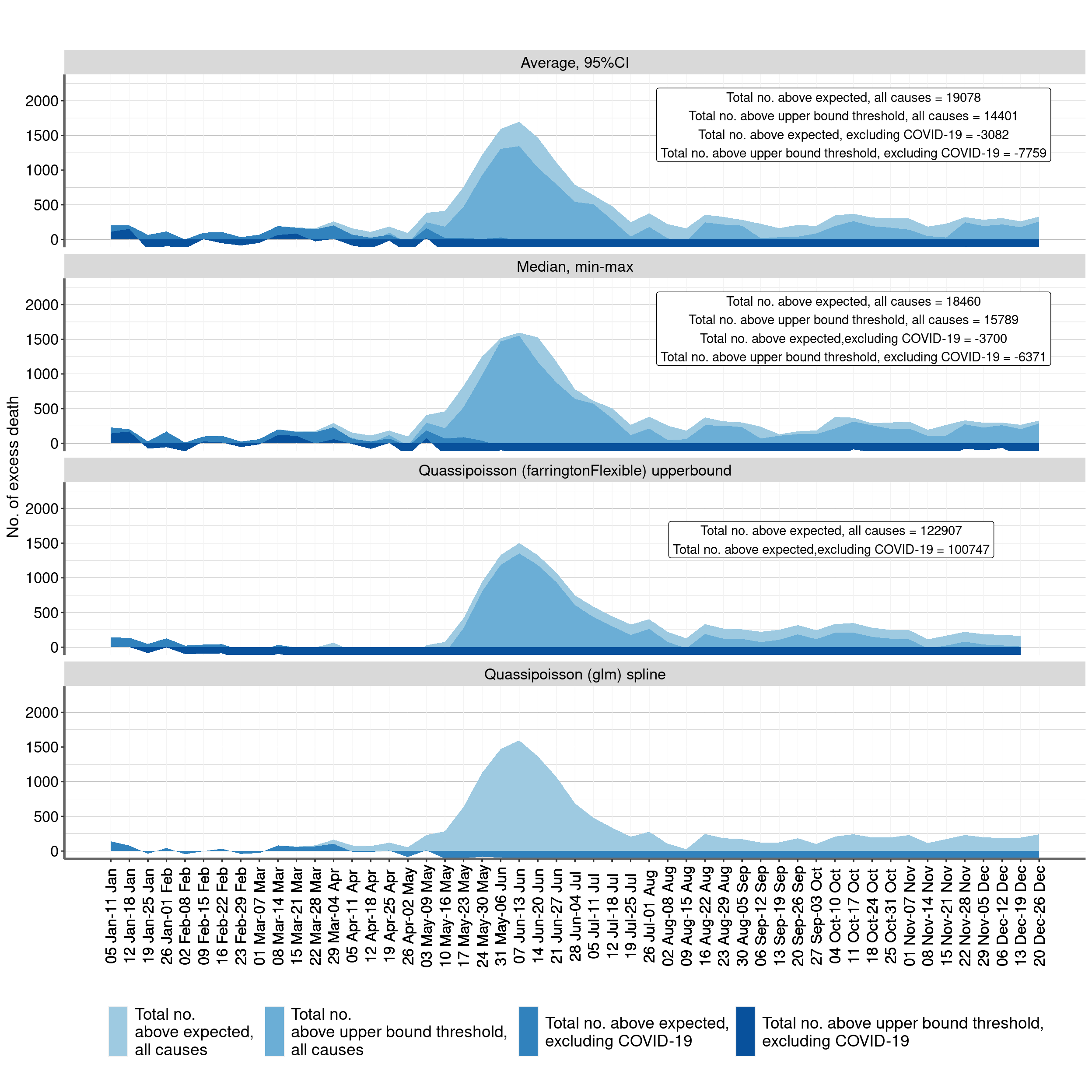
Figure 3: P score. Chile, 1 Jan -26 Dec of every year 2015 - 2020
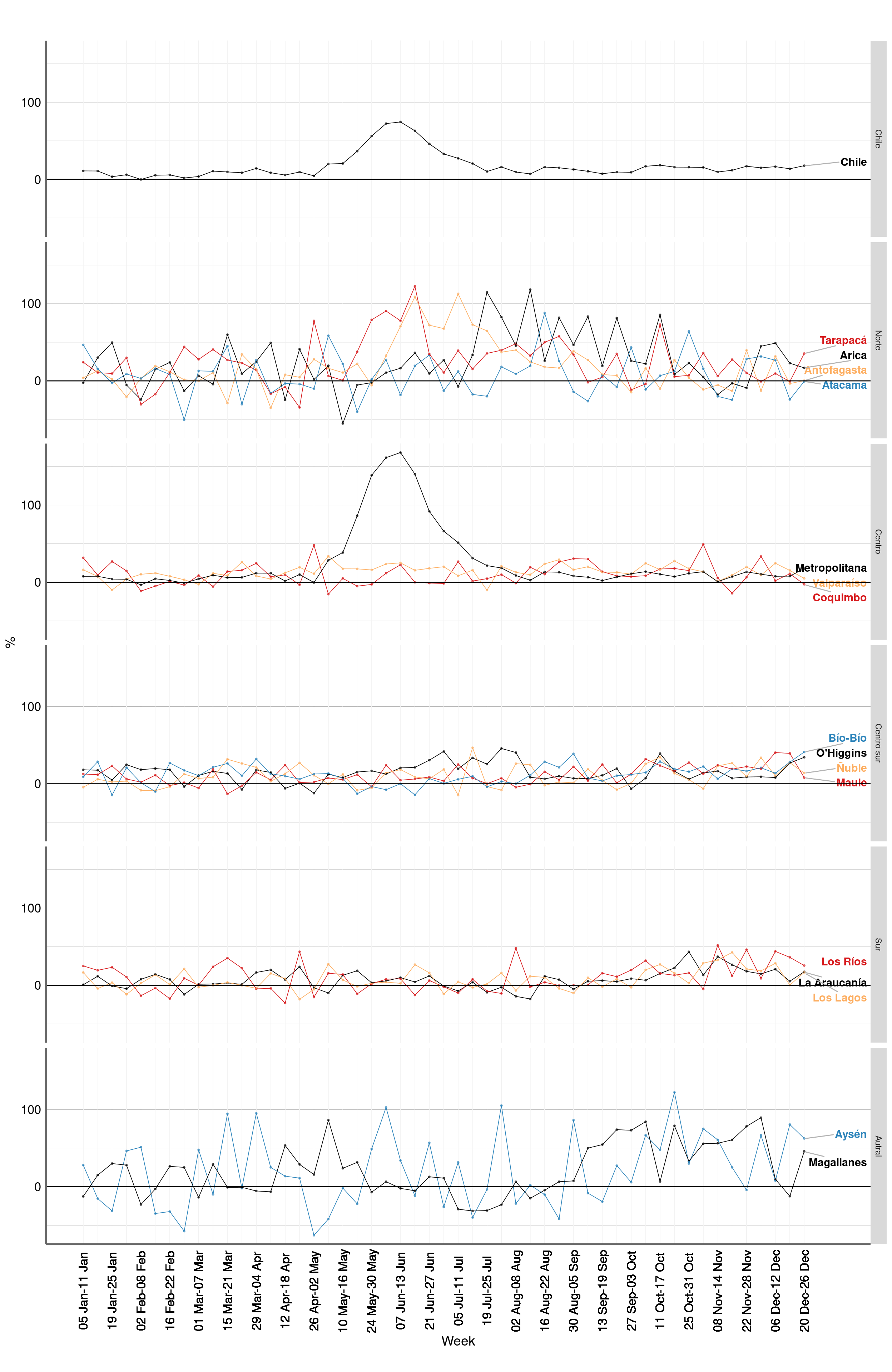
Figure 4: P score. Chile, 1 Jan -26 Dec of every year 2015 - 2020
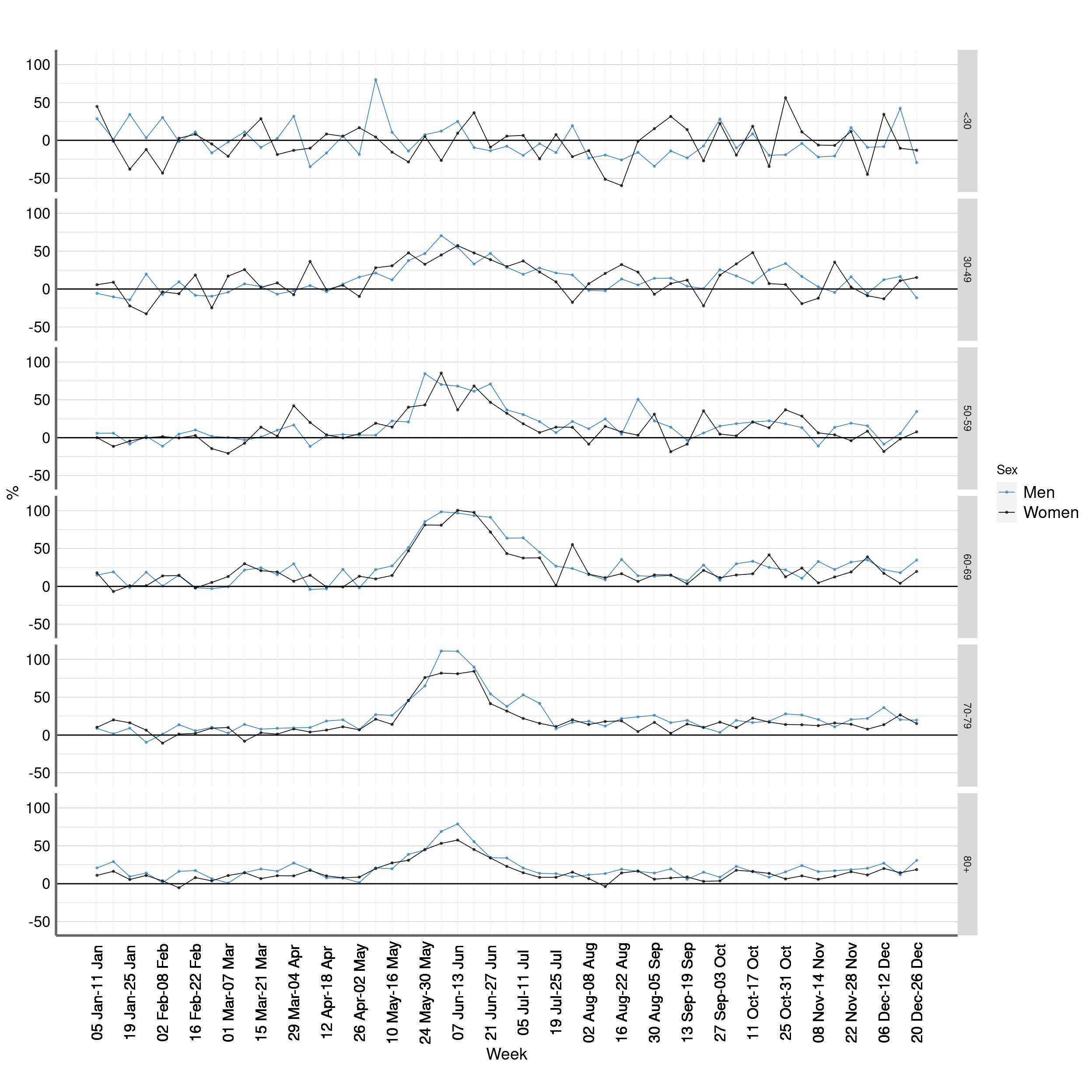
Figure 5: Causes of death. Chile, 1 Jan -26 Dec of every year 2015 - 2020
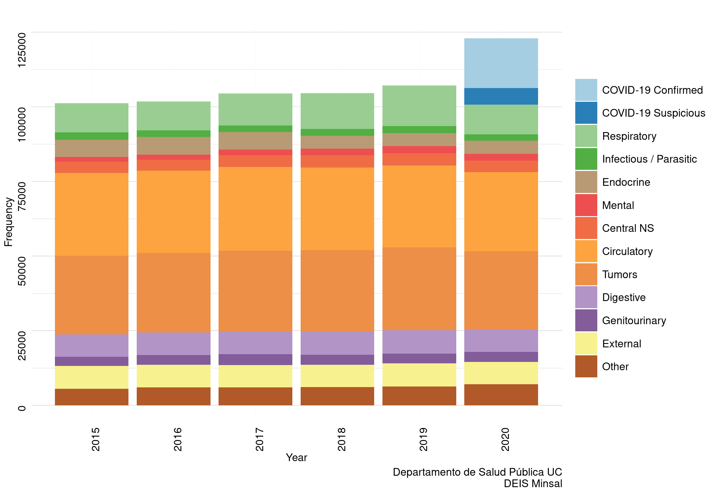
Table 1: Excess mortality in Chile 2020 using average and CI95% from 2015-2019
## [1] ""Table 2: Excess mortality in Chile 2020 using median, min and max from 2015-2019
## [1] ""Table 3: Excess mortality in Chile 2020 using Quasi-Poisson Regression from 2015-2019
## [1] ""Figure 6: p score farringtonflexible
## structure(c(2L, 3L, 4L, 1L, 5L, 6L, 7L, 8L, 9L, 10L, 11L, 12L,
## 13L, 14L, 15L, 16L, 17L, 18L, 19L, 20L, 21L, 22L, 23L, 24L), .Label = c("A00-B99 Infectious",
## "All \n", "All causes, excluding COVID-19 \n", "All causes, including suspected but not confirmed COVID-19 \n",
## "C00-D48 Neoplasms", "D50-D89 Blood", "E00-E90 Metabolic", "F00-F99 Mental",
## "G00-G99 Nervous", "H00-H59 Eye", "H60-H95 Ear", "I00-I99 Circulatory",
## "J00-J99 Respiratory", "K00-K93 Digestive", "L00-L99 Skin", "M00-M99 Musculoskeletal",
## "N00-N99 Genitourinary", "O00-O99 Pregnancy", "P00-P96 Perinatal",
## "Q00-Q99 Malformations", "R00-R99 No-classified", "S00-T98 External",
## "U07.1 COVID Confirmed", "U07.2 COVID Suspected"), class = "factor")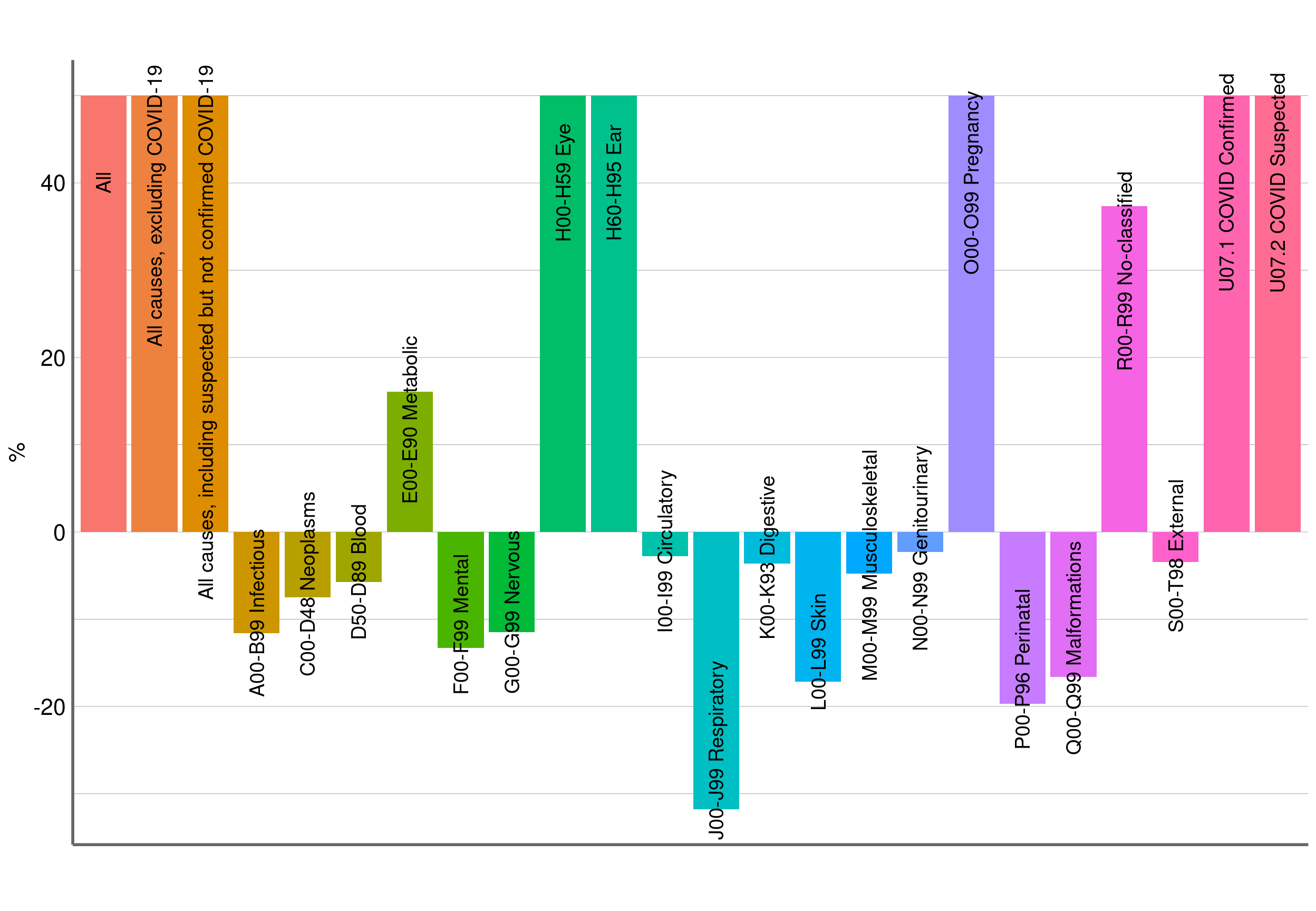
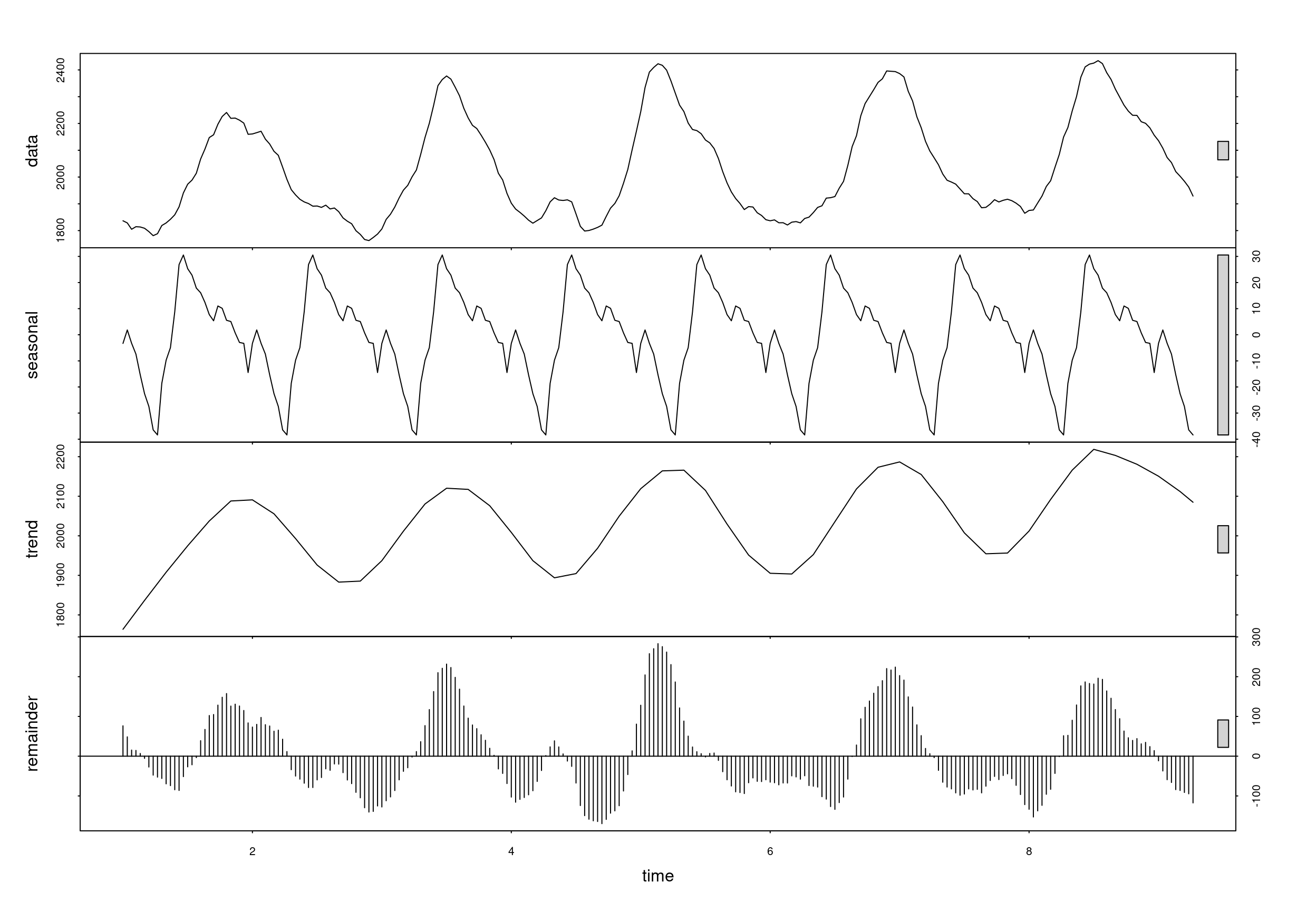
Linear regression time series ts